Overview

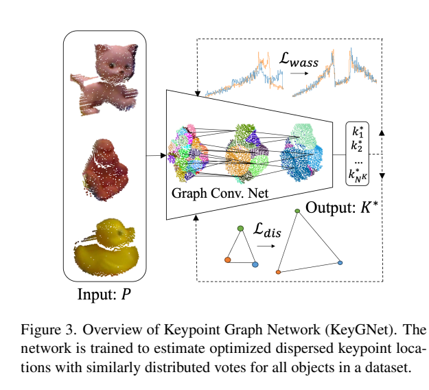
This addresses the issue of keypoint selection, by creating an optimal selection.

End-to-end

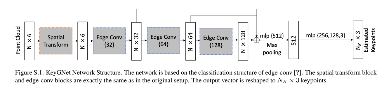
Input: $N\times6$ point cloud representing $(x,y,z,R,G,B)$

1. Spatial Transform
   1. Input point cloud through spatial transform, this normalizes the data in a canonical way so that we define all our input in the same “orientation”.
2. Edge conv:
   1. Run transformed data through three edge convolutions. These operate on the edges connecting the points in our data. This updates the features of each point w.r.t. the neighbouring points.
3. Output:
   1. Outputs a $N_{K}\times3$ vector which represent the keypoints we’re predicting.
4. Loss!
   1. We use Wasserstein loss, $\mathcal{L}_{wass}$, because it:
      1. Is more robust to small changes in the input
      2. Good for keypoint prediction as even when two compared distributions don’t overlap it still provides a good estimation.
      3. Here we apply gradient penalty to make predictions similar to each other rather than the ground truth.
   2. We use dispersion loss $\mathcal{L}_{dis}$ to:
      1. Make sure keypoints are well-dispersed
   3. Final loss: $\mathcal{L}=\alpha\mathcal{L}_{wass}+\beta\mathcal{L}_{dis}$