Problem

Suppose we have a sequence of RVs $X_{1},\dots,X_{n}$ which have the same marginal distribution. If we perform sample-by-sample scalar quantization, this yields the average MSE $$E\left[ \frac{1}{n}\sum_{i=1}^{n}(X_{i}-Q(X_{i}))^{2} \right]=E[(X_{i}-Q(X_{i}))^{2}]$$We observe that distortion stays the same whether or not our $X_{i}$’s have any interdependence. So since we aren’t exploiting the statistical interdependence between RVs we aren’t squeezing out the most out of our quantization that we should be.

Idea

To exploit the statistical interdependence we can form a linear prediction, $\hat{X}_{n}$, from the previous $m$ samples $$\tilde{X}_{n}=\sum_{i=1}^{m}a_{i}X_{n-i}$$and quantize the difference signal $$\begin{align*} e_{n}&=X_{n}-\tilde{X}_{n}\\ &=X_{n}-a_{1}X_{n-1}-\dots-a_{m}X_{n-m} \end{align*}$$

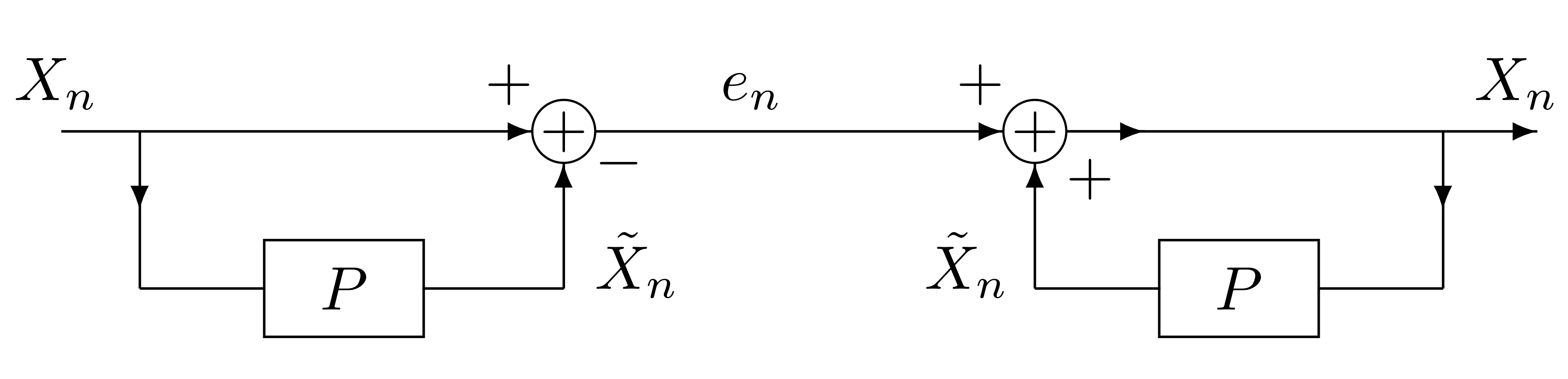
Let $P$ be the FIR Filter with transfer function $$P(z)=\sum_{i=1}^{m}a_{i}z^{-i}$$Without quantization the $X_{n}$ can be perfectly reconstructed:

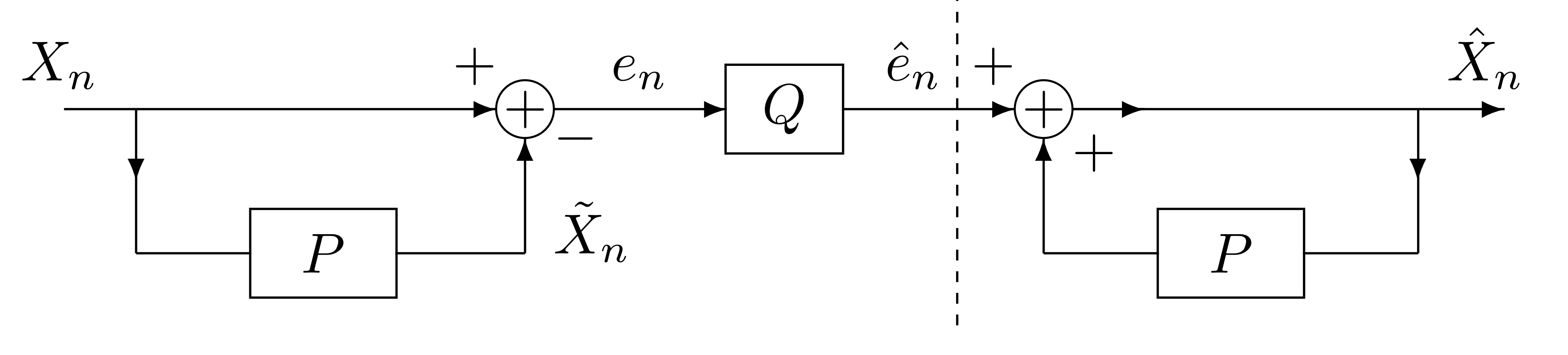
We see that since $e_{n}$ is less spread out in its output that it is easier to quantize. Adding quantization to the mix we now have our proposed scheme:

We see if quantization error is small then $e_{n}\approx \hat{e}_{n}\implies \hat{X}_{n}\approx X_{n}$. But in this structure we see the error accumulates.

Let $h_{n}$ denote the impulse response of the transfer function $\frac{1}{1-P(z)}$, also let $\hat{X}_{n}=\hat{e}_{n}*h_{n}$, $X_{n}=e_{n}*h_{n}$, and $X_{n}-\hat{X}_{n}=(e_{n}-\hat{e}_{n})*h_{n}$. Hence, $$\begin{align*} E[(X_{n}-\hat{X}_{n})^{2}]&=E[((e_{n}-\hat{e}_{n})*h_{n})^{2}]\\ &=E\left[ \left( \sum_{i=0}^{n}\smash[b]{\underbrace{ (e_{n-i}-\hat{e}_{n-i}) }_{\mathclap{e_{n-i}-Q(e_{n-i})} }}*h_{i} \right)^{2} \right] \vphantom{\underbrace{ (e_{n-i}-\hat{e}_{n-i}) }_{e_{n-i}-Q(e_{n-i}) }} \end{align*}$$We see that at time $n$ we depend on all past quantization errors $e_{i}-Q(e_{i})$! This means all our errors accumulate. We need a different structure, which brings us to Difference Quantization.

E2E

$$\begin{align*} \hat{X}_{n}&=\hat{e}_{n}+\tilde{X}_{n}\\ &=Q(e_{n})+\tilde{X}_{n}\\ &=Q(X_{n}-U_{n})+\tilde{X}_{n}\\ &=Q\left( X_{n}-\sum_{i=1}^{m}a_{i}\hat{X}_{n-i} \right)+\sum_{i=1}^{m}a_{i}\hat{X}_{n-i}\\ \end{align*}$$